Andy Maloney

sizing lactose 02

Posted by () in Open Notebook Science, powder_tapping on May 19, 2013

I went ahead and developed my own script to look at the 10th, 50th, and 90th percentiles for the particle sizing done on the SympaTEC HELOS laser diffractor device. As I suspected, the machine does in fact plot the cumulative distribution of particles and fits the data to a Sigmoid. It then calculates the 10th, 50th, and 90th percentiles and reports those values back to a txt file. The script is below the summary table. I will note that I got a NAN for one of the calculated measurements which, caused me to toss out that data point for my calculations. For completeness, I also removed it from the reported values.

Forgive the markdown table below, wordpress doesn’t recognize how to deal with markdown for some reason. It also doesn’t understand what WHITESPACE is supposed to mean. Nonetheless, it is clear that the machine is doing what one would expect as my calculated values are within error of the values reported. This is good as it is no longer a blackbox to me and I will report the values that it gives.

Pharmatose 150M
| Percentile | Reported Average | Reported STD | Calculated Ave | Calculated STD |
|:----------:|:----------------:|:------------:|:--------------:|:--------------:|
| 10th       | 121.9 µm         |  6.6 µm      | 117.1 µm       |  6.5 µm        |
| 50th       | 190.7 µm         | 11.4 µm      | 191.9 µm       | 11.8 µm        |
| 90th       | 268.2 µm         | 22.6 µm      | 260.0 µm       | 20.8 µm        |

SuperTab 11SD
| Percentile | Reported Average | Reported STD | Calculated Ave | Calculated STD |
|:----------:|:----------------:|:------------:|:--------------:|:--------------:|
| 10th       | 119.7 µm         |  7.9 µm      | 116.3 µm       |  6.1 µm        |
| 50th       | 187.9 µm         | 15.1 µm      | 189.1 µm       | 16.6 µm        |
| 90th       | 271.4 µm         | 39.9 µm      | 262.4 µm       | 32.9 µm        |

SuperTab 30GR
| Percentile | Reported Average | Reported STD | Calculated Ave | Calculated STD |
|:----------:|:----------------:|:------------:|:--------------:|:--------------:|
| 10th       | 117.9 µm         | 26.5 µm      | 117.9 µm       | 18.1 µm        |
| 50th       | 183.5 µm         | 21.0 µm      | 189.9 µm       | 13.4 µm        |
| 90th       | 257.4 µm         | 28.3 µm      | 256.4 µm       | 19.2 µm        |


# Import statements.
import numpy as np
from scipy.optimize import curve_fit

# Input data.
size = [ 4.50, 5.50, 6.50, 7.50, 9.00, 11.00, 13.00,
 15.50, 18.50, 21.50, 25.00, 30.00, 37.50, 45.00,
 52.50, 62.50, 75.00, 90.00, 105.00, 125.00, 150.00,
 180.00, 215.00, 255.00, 305.00, 365.00, 435.00, 515.00,
 615.00, 735.00, 875.00 ]

# Pharmatose 150M
pharmatose_150M_od43_63 = [
 2.16, 2.38, 2.54, 2.67, 2.82, 2.96, 3.07,
 3.17, 3.28, 3.37, 3.46, 3.59, 3.77, 3.94,
 4.10, 4.31, 4.67, 5.43, 6.96, 11.20, 21.73,
 41.64, 67.86, 89.30, 100.00, 100.00, 100.00, 100.00,
 100.00, 100.00, 100.00 ]
pharmatose_150M_od08_90 = [
 1.62, 1.87, 2.08, 2.26, 2.49, 2.73, 2.91,
 3.08, 3.20, 3.27, 3.27, 3.27, 3.27, 3.27,
 3.35, 3.52, 3.80, 4.40, 5.81, 10.75, 25.32,
 51.46, 81.69, 97.52, 100.00, 100.00, 100.00, 100.00,
 100.00, 100.00, 100.00 ]
pharmatose_150M_od15_83 = [
 2.27, 2.49, 2.63, 2.74, 2.84, 2.93, 2.93,
 2.93, 2.93, 2.93, 2.93, 2.93, 2.93, 2.93,
 3.01, 3.13, 3.36, 3.92, 5.31, 9.84, 21.84,
 42.60, 67.85, 88.46, 99.02, 100.00, 100.00, 100.00,
 100.00, 100.00, 100.00 ]
pharmatose_150M_od15_52 = [
 1.69, 1.90, 2.06, 2.18, 2.33, 2.47, 2.57,
 2.57, 2.57, 2.57, 2.57, 2.57, 2.57, 2.57,
 2.68, 2.81, 2.98, 3.38, 4.42, 8.12, 18.74,
 38.48, 63.38, 84.92, 94.39, 96.65, 100.00, 100.00,
 100.00, 100.00, 100.00 ]
pharmatose_150M_od09_31 = [
 2.25, 2.54, 2.77, 2.96, 3.17, 3.38, 3.53,
 3.66, 3.77, 3.84, 3.84, 3.84, 3.84, 3.92,
 4.05, 4.25, 4.55, 5.26, 7.09, 13.46, 29.42,
 53.34, 79.60, 94.53, 100.00, 100.00, 100.00, 100.00,
 100.00, 100.00, 100.00 ]
pharmatose_150M_od21_24 = [
 2.29, 2.53, 2.70, 2.82, 2.94, 3.03, 3.03,
 3.03, 3.03, 3.03, 3.03, 3.09, 3.23, 3.38,
 3.53, 3.73, 4.07, 4.78, 6.38, 11.15, 22.47,
 40.47, 61.63, 80.36, 94.20, 100.00, 100.00, 100.00,
 100.00, 100.00, 100.00 ]
pharmatose_150M_od13_58 = [
 2.42, 2.66, 2.82, 2.93, 3.05, 3.14, 3.14,
 3.14, 3.14, 3.14, 3.14, 3.14, 3.14, 3.14,
 3.22, 3.36, 3.60, 4.11, 5.23, 8.67, 18.17,
 36.99, 62.47, 83.56, 94.95, 100.00, 100.00, 100.00,
 100.00, 100.00, 100.00 ]
pharmatose_150M_od07_26 = [
 3.11, 3.51, 3.81, 4.03, 4.27, 4.48, 4.60,
 4.70, 4.70, 4.70, 4.70, 4.76, 4.87, 5.04,
 5.25, 5.57, 6.03, 6.97, 9.19, 16.09, 32.51,
 57.07, 81.43, 94.38, 100.00, 100.00, 100.00, 100.00,
 100.00, 100.00, 100.00 ]
pharmatose_150M_od15_40 = [
 2.57, 2.90, 3.15, 3.33, 3.51, 3.66, 3.75,
 3.75, 3.75, 3.75, 3.75, 3.80, 3.92, 4.06,
 4.19, 4.36, 4.59, 5.09, 6.23, 9.78, 19.14,
 36.31, 58.95, 82.39, 98.64, 100.00, 100.00, 100.00,
 100.00, 100.00, 100.00 ]
pharmatose_150M_od16_94 = [
 2.60, 2.89, 3.09, 3.22, 3.35, 3.44, 3.44,
 3.44, 3.44, 3.44, 3.44, 3.53, 3.66, 3.77,
 3.87, 4.02, 4.26, 4.73, 5.79, 9.07, 17.62,
 33.27, 53.49, 73.69, 89.55, 97.91, 100.00, 100.00,
 100.00, 100.00, 100.00 ]

pharmatose_150M_ave = [np.average(item) for item in
 zip(pharmatose_150M_od43_63, pharmatose_150M_od08_90,
 pharmatose_150M_od15_83, pharmatose_150M_od15_52,
 pharmatose_150M_od09_31, pharmatose_150M_od21_24,
 pharmatose_150M_od13_58, pharmatose_150M_od07_26,
 pharmatose_150M_od15_40, pharmatose_150M_od16_94)]
pharmatose_150M_std = [np.std(item) for item in
 zip(pharmatose_150M_od43_63, pharmatose_150M_od08_90,
 pharmatose_150M_od15_83, pharmatose_150M_od15_52,
 pharmatose_150M_od09_31, pharmatose_150M_od21_24,
 pharmatose_150M_od13_58, pharmatose_150M_od07_26,
 pharmatose_150M_od15_40, pharmatose_150M_od16_94)]

pharmatose_150M = [ pharmatose_150M_od43_63, pharmatose_150M_od08_90,
 pharmatose_150M_od15_83, pharmatose_150M_od15_52,
 pharmatose_150M_od09_31, pharmatose_150M_od21_24,
 pharmatose_150M_od13_58, pharmatose_150M_od07_26,
 pharmatose_150M_od15_40, pharmatose_150M_od16_94 ]

# SuperTab 11SD
supertab_11SD_od20_93 = [
 0.43, 0.50, 0.57, 0.63, 0.71, 0.81, 0.90,
 0.99, 1.10, 1.19, 1.29, 1.43, 1.65, 1.88,
 2.13, 2.49, 3.07, 4.27, 6.70, 13.32, 29.17,
 56.35, 84.37, 100.00, 100.00, 100.00, 100.00, 100.00,
 100.00, 100.00, 100.00 ]
supertab_11SD_od12_18 = [
 0.55, 0.61, 0.61, 0.61, 0.61, 0.61, 0.61,
 0.61, 0.61, 0.61, 0.68, 0.80, 0.99, 1.21,
 1.45, 1.81, 2.36, 3.43, 5.67, 12.27, 28.07,
 53.28, 81.44, 100.00, 100.00, 100.00, 100.00, 100.00,
 100.00, 100.00, 100.00 ]
supertab_11SD_od08_01 = [
 0.00, 0.07, 0.07, 0.07, 0.07, 0.07, 0.07,
 0.07, 0.07, 0.07, 0.16, 0.30, 0.54, 0.83,
 1.15, 1.63, 2.41, 3.92, 6.94, 15.44, 33.55,
 58.19, 83.75, 97.68, 100.00, 100.00, 100.00, 100.00,
 100.00, 100.00, 100.00 ]
supertab_11SD_od06_29 = [
 0.00, 0.06, 0.06, 0.06, 0.06, 0.06, 0.06,
 0.06, 0.06, 0.06, 0.15, 0.31, 0.56, 0.83,
 1.12, 1.53, 2.09, 2.92, 4.35, 8.68, 20.48,
 40.37, 63.77, 85.46, 99.23, 100.00, 100.00, 100.00,
 100.00, 100.00, 100.00 ]
supertab_11SD_od15_59 = [
 0.00, 0.06, 0.06, 0.06, 0.06, 0.06, 0.06,
 0.06, 0.06, 0.06, 0.16, 0.32, 0.59, 0.88,
 1.18, 1.59, 2.17, 3.14, 4.93, 9.76, 21.00,
 38.97, 60.11, 79.39, 94.27, 100.00, 100.00, 100.00,
 100.00, 100.00, 100.00 ]
supertab_11SD_od10_27 = [
 0.00, 0.06, 0.06, 0.06, 0.06, 0.06, 0.06,
 0.06, 0.06, 0.06, 0.14, 0.27, 0.49, 0.74,
 0.98, 1.29, 1.69, 2.39, 3.84, 8.10, 18.11,
 34.17, 53.57, 71.78, 85.51, 94.19, 100.00, 100.00,
 100.00, 100.00, 100.00 ]
supertab_11SD_od09_51 = [
 0.61, 0.76, 0.90, 1.04, 1.24, 1.51, 1.75,
 2.03, 2.32, 2.57, 2.85, 3.25, 3.86, 4.46,
 4.99, 5.60, 6.31, 7.52, 10.15, 17.87, 34.59,
 58.89, 83.86, 100.00, 100.00, 100.00, 100.00, 100.00,
 100.00, 100.00, 100.00 ]
supertab_11SD_od07_94 = [
 0.52, 0.60, 0.60, 0.60, 0.60, 0.60, 0.60,
 0.70, 0.81, 0.92, 1.04, 1.21, 1.50, 1.81,
 2.14, 2.61, 3.26, 4.33, 6.32, 11.81, 24.04,
 42.31, 63.21, 81.04, 92.89, 100.00, 100.00, 100.00,
 100.00, 100.00, 100.00 ]
supertab_11SD_od08_40 = [
 0.51, 0.59, 0.59, 0.59, 0.59, 0.59, 0.59,
 0.59, 0.59, 0.69, 0.82, 1.01, 1.32, 1.63,
 1.93, 2.31, 2.80, 3.64, 5.22, 9.51, 19.31,
 34.87, 53.46, 71.73, 86.80, 96.02, 100.00, 100.00,
 100.00, 100.00, 100.00 ]

supertab_11SD_ave = [np.average(item) for item in
 zip(supertab_11SD_od20_93, supertab_11SD_od12_18,
 supertab_11SD_od08_01, supertab_11SD_od06_29,
 supertab_11SD_od15_59, supertab_11SD_od10_27,
 supertab_11SD_od09_51, supertab_11SD_od07_94,
 supertab_11SD_od08_40) ]
supertab_11sd_std = [np.std(item) for item in
 zip(supertab_11SD_od20_93, supertab_11SD_od12_18,
 supertab_11SD_od08_01, supertab_11SD_od06_29,
 supertab_11SD_od15_59, supertab_11SD_od10_27,
 supertab_11SD_od09_51, supertab_11SD_od07_94,
 supertab_11SD_od08_40)]

supertab_11SD = [ supertab_11SD_od20_93, supertab_11SD_od12_18,
 supertab_11SD_od08_01, supertab_11SD_od06_29,
 supertab_11SD_od15_59, supertab_11SD_od10_27,
 supertab_11SD_od09_51, supertab_11SD_od07_94,
 supertab_11SD_od08_40 ]

# SuperTab 30GR
supertab_30GR_od05_40 = [
 0.89, 0.96, 0.96, 0.96, 0.96, 0.96, 0.96,
 0.96, 0.96, 0.96, 0.96, 0.96, 1.03, 1.14,
 1.26, 1.43, 1.63, 1.90, 2.53, 4.99, 13.15,
 30.51, 55.09, 80.77, 98.84, 100.00, 100.00, 100.00,
 100.00, 100.00, 100.00 ]
supertab_30GR_od14_59 = [
 0.82, 0.91, 0.91, 0.91, 0.91, 0.91, 0.91,
 0.91, 0.91, 0.91, 0.99, 1.11, 1.29, 1.47,
 1.64, 1.88, 2.23, 2.82, 3.96, 7.42, 17.30,
 37.26, 64.08, 86.29, 97.81, 100.00, 100.00, 100.00,
 100.00, 100.00, 100.00 ]
supertab_30GR_od14_16 = [
 0.81, 0.90, 0.90, 0.90, 0.90, 0.90, 0.90,
 0.90, 0.90, 0.90, 0.97, 1.07, 1.23, 1.40,
 1.57, 1.83, 2.19, 2.83, 4.08, 8.10, 19.27,
 38.78, 62.03, 80.56, 93.90, 100.00, 100.00, 100.00,
 100.00, 100.00, 100.00 ]
supertab_30GR_od12_68 = [
 1.11, 1.23, 1.32, 1.32, 1.32, 1.32, 1.32,
 1.32, 1.32, 1.32, 1.41, 1.55, 1.76, 2.01,
 2.29, 2.71, 3.30, 4.15, 5.64, 10.08, 22.32,
 43.58, 68.81, 86.73, 96.04, 99.37, 100.00, 100.00,
 100.00, 100.00, 100.00 ]
supertab_30GR_od19_84 = [
 1.08, 1.19, 1.28, 1.28, 1.28, 1.28, 1.28,
 1.28, 1.28, 1.28, 1.37, 1.50, 1.70, 1.91,
 2.14, 2.45, 2.89, 3.59, 4.96, 9.26, 21.13,
 42.65, 69.46, 90.32, 100.00, 100.00, 100.00, 100.00,
 100.00, 100.00, 100.00 ]
supertab_30GR_od16_64 = [
 1.34, 1.48, 1.59, 1.68, 1.78, 1.88, 1.97,
 1.97, 1.97, 2.06, 2.16, 2.30, 2.52, 2.75,
 2.98, 3.30, 3.73, 4.44, 5.85, 10.46, 23.76,
 47.74, 76.14, 92.11, 97.37, 100.00, 100.00, 100.00,
 100.00, 100.00, 100.00 ]
supertab_30GR_od07_38 = [
 8.09, 9.59, 10.86, 11.92, 13.20, 14.50, 15.46,
 6.35, 17.12, 17.71, 18.27, 18.98, 20.05, 21.20,
 2.48, 24.29, 26.55, 29.80, 34.86, 45.30, 62.11,
 80.83, 93.74, 100.00, 100.00, 100.00, 100.00, 100.00,
 100.00, 100.00, 100.00 ]
supertab_30GR_od22_13 = [
 1.32, 1.48, 1.60, 1.70, 1.82, 1.93, 2.02,
 2.12, 2.12, 2.21, 2.32, 2.46, 2.68, 2.90,
 3.14, 3.47, 3.93, 4.70, 6.09, 10.07, 20.37,
 38.47, 60.39, 79.95, 92.87, 98.84, 100.00, 100.00,
 100.00, 100.00, 100.00 ]
supertab_30GR_od14_21 = [
 1.99, 2.23, 2.41, 2.56, 2.74, 2.92, 3.06,
 3.20, 3.34, 3.46, 3.59, 3.78, 4.06, 4.36,
 4.65, 5.03, 5.49, 6.19, 7.54, 11.87, 24.41,
 48.74, 80.55, 98.71, 100.00, 100.00, 100.00, 100.00,
 100.00, 100.00, 100.00 ]
supertab_30GR_od09_15 = [
 3.94, 4.61, 5.17, 5.65, 6.22, 6.80, 7.23,
 7.62, 7.97, 8.25, 8.53, 8.89, 9.44, 10.01,
 10.60, 11.41, 12.38, 13.78, 16.37, 23.89, 41.22,
 66.35, 88.63, 98.00, 100.00, 100.00, 100.00, 100.00,
 100.00, 100.00, 100.00 ]

supertab_30GR_ave = [np.average(item) for item in
 zip(supertab_30GR_od05_40, supertab_30GR_od14_59,
 supertab_30GR_od14_16, supertab_30GR_od12_68,
 supertab_30GR_od19_84, supertab_30GR_od16_64,
 supertab_30GR_od07_38, supertab_30GR_od22_13,
 supertab_30GR_od14_21, supertab_30GR_od09_15) ]
supertab_30GR_std = [np.std(item) for item in
 zip(supertab_30GR_od05_40, supertab_30GR_od14_59,
 supertab_30GR_od14_16, supertab_30GR_od12_68,
 supertab_30GR_od19_84, supertab_30GR_od16_64,
 supertab_30GR_od07_38, supertab_30GR_od22_13,
 supertab_30GR_od14_21, supertab_30GR_od09_15) ]

supertab_30GR = [ supertab_30GR_od05_40, supertab_30GR_od14_59,
 supertab_30GR_od14_16, supertab_30GR_od12_68,
 supertab_30GR_od19_84, supertab_30GR_od16_64,
 supertab_30GR_od22_13,
 supertab_30GR_od14_21, supertab_30GR_od09_15 ]

# Define the Sigmoidal function.
def sigmoid(x, a, b, k, t):
 """ Sigmoidal function.
 x = Input data.
 a = Minimum value of input data.
 b = Maximum value of input data.
 k = Midpoint of the Sigmoid.
 t = Rate of increase.
 """
 y = a + (b/(1 + np.exp((k - x)/t)))
 return y

# Get the 10, 50, and 90th percentiles.
pharmatose_150M_percentiles = []
for item in pharmatose_150M:
 popt, pcov = curve_fit(sigmoid, size, item)
 _10 = popt[2] - popt[3]*np.log(popt[1]/(10 - popt[0]) - 1)
 _50 = popt[2] - popt[3]*np.log(popt[1]/(50 - popt[0]) - 1)
 _90 = popt[2] - popt[3]*np.log(popt[1]/(90 - popt[0]) - 1)
 temp = _10, _50, _90
 pharmatose_150M_percentiles.append(temp)
supertab_11SD_percentiles = []
for item in supertab_11SD:
 popt, pcov = curve_fit(sigmoid, size, item)
 _10 = popt[2] - popt[3]*np.log(popt[1]/(10 - popt[0]) - 1)
 _50 = popt[2] - popt[3]*np.log(popt[1]/(50 - popt[0]) - 1)
 _90 = popt[2] - popt[3]*np.log(popt[1]/(90 - popt[0]) - 1)
 temp = _10, _50, _90
 supertab_11SD_percentiles.append(temp)
supertab_30GR_percentiles = []
for item in supertab_30GR:
 popt, pcov = curve_fit(sigmoid, size, item)
 _10 = popt[2] - popt[3]*np.log(popt[1]/(10 - popt[0]) - 1)
 _50 = popt[2] - popt[3]*np.log(popt[1]/(50 - popt[0]) - 1)
 _90 = popt[2] - popt[3]*np.log(popt[1]/(90 - popt[0]) - 1)
 temp = _10, _50, _90
 supertab_30GR_percentiles.append(temp)

# Create a list of the generated percentile values.
pharmatose_150M_10 = [ 119.34, 121.96, 125.33, 129.43, 114.13, 120.18, 128.50,
 107.36, 125.58, 127.73 ]
pharmatose_150M_50 = [ 191.16, 178.32, 190.26, 196.19, 175.81, 195.76, 197.87,
 171.37, 201.16, 208.96 ]
pharmatose_150M_90 = [ 258.28, 236.00, 262.29, 281.83, 242.86, 289.82, 283.27,
 241.46, 278.42, 308.22 ]
pharmatose_150M_reported = [ pharmatose_150M_10, pharmatose_150M_50,
 pharmatose_150M_90 ]

supertab_11SD_10 = [ 114.96, 118.13, 112.20, 127.81, 125.54, 129.74, 104.16, 118.42, 126.26 ]
supertab_11SD_50 = [ 172.99, 176.09, 170.03, 194.41, 198.26, 208.57, 169.02, 192.88, 208.49 ]
supertab_11SD_90 = [ 229.41, 233.45, 232.95, 271.49, 290.66, 336.04, 230.22, 292.81, 325.82 ]
supertab_11SD_reported = [ supertab_11SD_10, supertab_11SD_50,
 supertab_11SD_90 ]

supertab_30GR_10 = [ 140.35, 131.52, 129.25, 124.65, 126.56, 123.02,
 124.67, 116.38, 44.88 ] # 5.82
supertab_30GR_50 = [ 207.76, 196.63, 196.89, 188.90, 189.60, 182.79, 131.99, 198.41, 181.39, 160.48 ]
supertab_30GR_90 = [ 280.54, 271.11, 290.39, 272.56, 254.39, 249.72, 204.86, 293.91, 235.82, 220.86 ]
supertab_30GR_reported = [ supertab_30GR_10, supertab_30GR_50,
 supertab_30GR_90 ]

for i in range(0, 3):
 rept_ave = np.average(pharmatose_150M_reported[i])
 calc_ave = np.average([item[i] for item in pharmatose_150M_percentiles])
 rept_std = np.std(pharmatose_150M_reported[i])
 calc_std = np.std([item[i] for item in pharmatose_150M_percentiles])
 print 'Calculated average for Pharmatose 150M = %f' % calc_ave
 print 'Reported average for Pharmatose 150M = %f' % rept_ave
 print 'Calculated STD for Pharmatose 150M = %f' % calc_std
 print 'Reported STD for Pharmatose 150M = %f' % rept_std

for i in range(0, 3):
 rept_ave = np.average(supertab_11SD_reported[i])
 calc_ave = np.average([item[i] for item in supertab_11SD_percentiles])
 rept_std = np.std(supertab_11SD_reported[i])
 calc_std = np.std([item[i] for item in supertab_11SD_percentiles])
 print 'Calculated average for SuperTab 11SD = %f' % calc_ave
 print 'Reported average for SuperTab 11SD = %f' % rept_ave
 print 'Calculated STD for SuperTab 11SD = %f' % calc_std
 print 'Reported STD for SuperTab 11SD = %f' % rept_std

for i in range(0, 3):
 rept_ave = np.average(supertab_30GR_reported[i])
 calc_ave = np.average([item[i] for item in supertab_30GR_percentiles])
 rept_std = np.std(supertab_30GR_reported[i])
 calc_std = np.std([item[i] for item in supertab_30GR_percentiles])
 print 'Calculated average for SuperTab 30GR = %f' % calc_ave
 print 'Reported average for SuperTab 30GR = %f' % rept_ave
 print 'Calculated STD for SuperTab 30GR = %f' % calc_std
 print 'Reported STD for SuperTab 30GR = %f' % rept_std

Leave a comment

sizing lactose 01

Posted by () in Open Notebook Science, powder_tapping on May 18, 2013

Particle sizing

I was able to size the lactose particles after sieving using the SympaTEC HELOS laser diffractor in the lab. I unfortunately had to do this step multiple times as I was having some difficulty interpreting the results. Nonetheless, I believe I understand how the device works now.

The sizer uses a laser to illuminate particles that are suspended in mineral oil that has 1% Span-85 in it. The laser is collimated and has a beam width of about 2 cm. A lens is then used to focus the light from the sample onto a detector. The detector is placed in the Fourier plane of the lens in order to detect diffraction patterns from the particles. Using Fraunhofer diffraction theory, a particle size is estimated from its diffraction pattern.

What caused my initial hesitation about the results was that I was told to not put a lot of particles in the cuvette—so I didn’t. However, I was told to add more particles to the cuvette and take successive measurements. I found documentation on the computer that states one should shoot for a 10–15% optical density which, at the time of my first run with the machine, I had no clue as to what that meant. My main cause of confusion and why I redid the sizing was when I added particles to the cuvette, it caused the sizing results to shift slightly.

My second go with the machine allowed for more clarity. I understand the caution for not putting a ton of particles in the cuvette since you don’t want to saturate the detector. If there are too many particles, than the detector (which I’m assuming is nothing more than a camera with multiple arrays) is unable to detect individual diffraction patterns through the software. I did oversaturate the detector once but, I just waited a couple of minutes till the particles settled in the cuvette. I then retook the measurement and sure enough, the detector wasn’t saturated. Of course doing this skews the particle size results as the detector is detecting particles small enough that stayed in solution. The sizer indicates the “optical density” of a measurement and I believe this is a measure of the turbidity of the solution in the cuvette. I was able to get it as high as 44% optical density without the software complaining.

The data I obtained shifted dependent upon the time in which particles were allowed to be in the cuvette—i.e. larger ones sank. So, I made sure to load the cuvette with tons of particles, wait till it was able to detect them, and then took measurements as particles sunk. I also added particles to the cuvette over time adding small amounts as was instructed for me to do. Doing this gave a spread in sizing that I’m assuming comes from a spread in particles after sieving.

The SympaTEC software gives a plot of sizing data and shows the 10th, 50th, and 90th percentile of the sizes. I believe it is doing this by fitting a Sigmoid to the size data and finding on the curve the corresponding percentiles. This data is of course plotted in a proprietary .bmp format that is completely useless. So, I’m working on a script to plot the data which, thankfully was output in a txt file. For all intents and purposes I believe using the data that was output by the device is sufficient for sizing purposes. I’m just wanting to have a little fun with the data it gave me.

1 Comment

sieving analysis

Posted by () in Open Notebook Science, powder_tapping on May 18, 2013

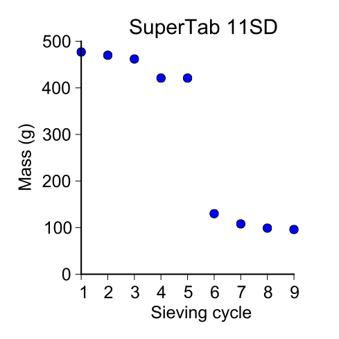
I finished my sieving analysis and writeup for it. Below is the python script that I used to plot the data shown in the graphs below. I don’t know why but wordpress is removing my white space formatting.


# Import statements.
 import matplotlib.pyplot as plt
 from matplotlib import rcParams

# Change the figure size and font used.
 rcParams['font.sans-serif'] = 'Arial'
 rcParams['figure.figsize'] = [3.27, 3.27]
 rcParams['xtick.direction'] = 'out'
 rcParams['ytick.direction'] = 'out'

# Input data. Values are in grams.
 pharmatose150M = [ 205, 165, 103, 90, 85, 81, 81, 78, 75 ]
 supertab11SD = [ 477, 470, 462, 421, 421, 130, 108, 99, 96 ]
 supertab30GR = [ 246, 239, 236, 234, 218, 209, 202, 200 ]

# Generate the x-axis.
 sieve_cycle = [ 1, 2, 3, 4, 5, 6, 7, 8, 9 ]

# Plot the data.
 def plot_data(x, y, marker_type, marker_size, x_label, y_label, title):
 """ Plots the input data.
 x = x-data
 y = y-data
 marker_type = Marker type of the plot.
 marker_size = Marker size of the plot.
 x_label = x-axis label.
 y_label = y-axis label.
 title = Title of the plot.
 """
 # Initialize a figure.
 fig = plt.figure()
 ax = fig.add_subplot(1, 1, 1)
 # Add labels.
 ax.set_xlabel(x_label)
 ax.set_ylabel(y_label)
 ax.set_title(title)
 # Fix the x-axis limit.
 ax.set_xlim([1, 10])
 # Modify the spines so that the top and right spines are not visible.
 ax.xaxis.set_ticks_position('bottom')
 ax.yaxis.set_ticks_position('left')
 ax.spines['right'].set_visible(False)
 ax.spines['top'].set_visible(False)
 ax.spines['left'].set_smart_bounds(True)
 ax.spines['bottom'].set_smart_bounds(True)
 #ax.spines['left'].set_position(('axes', -0.01))
 # Plot the data.
 data = ax.plot(x, y, marker_type, marker_size)
 for artist in data:
 artist.set_clip_on(False)
 fig.tight_layout()
 fig.savefig(title.lower().replace(' ', '') + '.pdf')

plot_data(sieve_cycle, pharmatose150M, 'o', 3, 'Sieve cycle', 'Mass (g)',
 'Pharmatose 150M')
 plot_data(sieve_cycle, supertab11SD, 'o', 3, 'Sieve cycle', 'Mass (g)',
 'SuperTab 11SD')
 plot_data(sieve_cycle[:-1], supertab30GR, 'o', 3, 'Sieve cycle', 'Mass (g)',
 'SuperTab 30GR')

Leave a comment

sieving lactose 03

Posted by () in Open Notebook Science, powder_tapping on May 5, 2013

Last time I did a bulk sieving of the powders in order to fractionate them into different distributions of grain sizes. From this initial sieving, I saw that the largest amount of powder in each of the sieved sizes was the 125–150 µm range. If the Pharmatose 150M lactose took approximately the same number of sieving cycles as the SuperTabs than I wouldn’t be doing this extra sieving step, however, because it took 8 cycles I am not convinced that the sieving is complete enough to give large cutoffs for the 125–150 µm size range. This is why I have decided to sieve each of the 125–150 µm sizes again to ensure that sieving is producing a strong cutoff between sizes. Like before, I’ve set up the following sieves:

Lid
250 µm
125 µm
75 µm
Bucket

this time ignoring the 45 µm sieve since it has a hole in it. I put the 125–150 µm size range in the top sieve and let it shake for 30 minutes. I’m only interested in the 125–250 µm range so this is the only one that I will be measuring.

SuperTab 30GR

Initial conditions:

2014-05-04
Temperature = 22.9˚C
Relative humidity = 22%

My first sieving for the second sieve cycle was:

125–250 µm = 218 g

I’ll note that the powder seemed to be have somewhat of a charge to it and as such, seemed to cling to the sieve. As seen in a previous post, this weight is significantly different than the one I ended with so, time for another sieve cycle.

My second sieving for the second sieve cycle was:

125–250 µm = 209 g

My third sieving for the second sieve cycle was:

125–250 µm = 202 g

My fourth sieving for the second sieve cycle was:

125–250 µm = 200 g

Pharmatose 150M

My first sieving for the second sieve cycle was:

125–250 µm = 75 g

Since the last sieving of the Pharmatose 150M was at 78 g, this change is within the 1–5% weight change and thus I will not be sieving it more.

SuperTab 11SD

I separated the SuperTab 125–250 µm fraction because it was quite large. So I started off with about 150 g of it in the sievers.

My first sieving for the second sieve cycle was:

125–250 µm = 130 g

My second sieving for the second sieve cycle was:

125–250 µm = 108 g

My third sieving for the second sieve cycle was:

125–250 µm = 99 g

My fourth sieving for the second sieve cycle was:

125–250 µm = 96 g

The powders are now within the arbitrarily decided 1–5% change of weight between sieving cycles. The next step is to size the particles to see if they actually are within these ranges.

Leave a comment

sieving lactose 02

Posted by () in Open Notebook Science, powder_tapping on April 30, 2013

Continuing from yesterday, I am sieving the SuperTab 11SD lactose. Except today I have split the large fraction between 125–250 µm into two batches. I will sieve both batches for 30 minutes.

23.1˚C
47% relative humidity

SuperTab 11SD

My fourth sieving obtained the following:

> 250 µm = 8 g
125–250 µm = 421 g
75–125 µm = 14 g
45–75 µm = < 1 g
< 45 µm = 37 g

My fifth sieving obtained the following:

> 250 µm = 7 g
125–250 µm = 421 g
75–125 µm = 13 g
45–75 µm = < 1 g
< 45 µm = 39 g

This looks like a good stopping point as I’m wanting to use the 125–250 µm fraction and it hasn’t change appreciably.

Pharmatose 150M

This powder is much more cohesive than the SuperTab powders. I’ll also note that the bag of lactose, when received, was open in the jar. This is fine as the powder was exposed to the elements during shipping and thus may have more moisture content in it than the other powders. A comparison can now be made between powders and their moisture content—dependent on if the moisture content is greater in the pharmatose powder.

My first sieving obtained the following:

> 250 µm = 9 g
125–250 µm = 205 g
75–125 µm = 191 g
45–75 µm = 21 g
< 45 µm = 68 g

My second sieving obtained the following:

> 250 µm = 5 g
125–250 µm = 165 g
75–125 µm = 209 g
45–75 µm = 4 g
< 45 µm = 109 g

My third sieving obtained the following:

> 250 µm = 5 g
125–250 µm = 103 g
75–125 µm = 223 g
45–75 µm = 4 g
< 45 µm = 153 g

Sieving the Pharmatose 150M is _very_ different than sieving the SuperTab powders. There seems to be a large amount of grains that are less than 45 µm in the batch and are for some reason getting stuck in the various sieves and powders in the sieves probably due to cohesiveness. Not sure though. I am making sure that the sieves are clear between each cycle. I suspect that more sieving sessions will refine the particle distributions but, I may end up with a bunch of powder with particle sizes less than 45 µm. I hope that the particles in the 125–250 µm range are for the most part separated nicely as this is the fraction that I wish to use in further experiments.

My fourth sieving obtained the following:

> 250 µm = 5 g
125–250 µm = 90 g
75–125 µm = 201 g
45–75 µm = 14 g
< 45 µm = 175 g

As suspected, I lost more in the 125–250 µm range. There still seems to be enough for this project but I need to go through another cycle since there was a 10% change in weight between sieving 3 and 4. I’ll also note that the powder in the 125-250 µm range is flowing better out of the sieve and into the jar I am putting it in. I’m guessing because the number of smaller particles in this fraction are becoming less.

My fifth sieving obtained the following:

> 250 µm = 5 g
125–250 µm = 85 g
75–125 µm = 171 g
45–75 µm = 2 g
< 45 µm = 207 g

My sixth sieving obtained the following:

> 250 µm = 5 g
125–250 µm = 81 g
75–125 µm = 144 g
45–75 µm = 2 g
< 45 µm = 235 g

I will do one more since the diference between the 75–125 is still above a 10% change in weight. I do know why my 45–75 µm fraction is always small, it’s because there is a rip in the sieve where it meets the holder. No wonder why I was not getting any in that fraction for all the powders. This isn’t a problem, it just means that my smallest fraction is actually < 75 µm and not < 45 µm. I’ll fix my notes after the seventh sieving just so I stay consistent with what I started, i.e. so I don’t mess up with this final sieve.

My seventh sieving obtained the following:

> 250 µm = 5 g
125–250 µm = 81 g
75–125 µm = 144 g
45–75 µm = 2 g
< 45 µm = 235 g

My eighth sieving obtained the following:

> 250 µm = 4 g
125–250 µm = 78 g
75–125 µm = 119 g
45–75 µm = X g
< 45 µm = 262 g

I have to admit that this was fairly tedious and left me guessing if the sieving actually worked. I am wanting to ensure that the distribution in sizes of the particles are what I think they are so I may end up sieving the 125–250 µm fraction for all lactose types again and ensuring that the weight change between sieving cycles is less than 5%. I want to use the 125–250 µm particle size range as all three powders have > 50 g of powder in that range. So, I think I will end up sieving this range again just to make sure that the particle distribution is as narrow as I think it should be. Of course I will need to size the particles after the sieving process is complete.

I will also note that the Pharmatose 150M lactose in the 125–250 µm size range was pretty cohesive when I was trying to empty the powder out of the sieves for the first couple of cycles. After about the 5th one, the particles started flowing out much more smoothly and I think this is because the smaller particles were leaving this fraction. Still, I think I need to sieve the particles some more next time I’m in.

1 Comment

sieving lactose

Posted by () in Open Notebook Science, powder_tapping on April 29, 2013

Introduction

This project is a continuation of initial experiments done by Sarah, Damian and Jihyun. The experiments that I will conduct are basic refinements from their initial experiments and will serve as a metric for more standardized tests that can be done with powders. The goal will be to investigate the gold standards for powder characterization for pharmaceutical excipients and compare them to our novel tapping apparatus.

Sieving

I received lactose powder from DFEPharma on 2013-04-25 and am in the process of sieving it. I received three types of powders:

where GR=granulated, SD=spray dried, and M=milled lactose types. My process for sieving consists of the following steps:

Weigh the initial amount of powder received.
Stack the following sieves from top (1) to bottom (6):
1. Lid
2. 250 µm sieve
3. 125 µm sieve
4. 75 µm sieve
5. 45 µm sieve
6. Collection bucket.
Place all the powder in the top most sieve and let the sieving machine go for 30 minutes—this is the first sieving. The machine is a Tyler RX-24 Portable Sieve Shaker.
Take each fraction and weigh the amount of powder in each sieve.
Return the powder to its respective sieve and allow the machine to shake for 30 more minutes.
Repeat until there is no appreciable weight change between sieves for each fraction.

The sieving machine can be seen in action in the below video. It’s a loud machine but, very effective at what it does.

SuperTab 30GR

I started with the SuperTab 30GR granulated lactose powder. The ambient climate here in Austin for 2013-04-29 and my initial powder weight conditions are:

Temperature = 23.5˚C
Relative humidity = 47%
Initial amount of powder = 498 g
Powder name: Monohydrate Lactose USP/NF, Ph. Eur., JP
Product code: 42320-6460
Product date: 04-2012
Charge Number: 10637764
ME/SU number: 5633687
Expiration date: 03-2015
Drum number: 854

I had some difficulty starting the machine due to not tightening the clamps that hold the sieve down enough, however, things are moving smoothly now. For my first sieve, I obtained the following fractions:

> 250 µm = 42 g
125–250 µm = 246 g
75–125 µm = 122 g
45–75 µm < 1 g
< 45 µm = 84 g

where the weight measurements are ±1 g. My second sieve obtained the following fractions:

> 250 µm = 40 g
125–250 µm = 239 g
75–125 µm = 126 g
45–75 µm < 1 g
< 45 µm = 88 g

My third sieving obtained the following:

> 250 µm = 39 g
125–250 µm = 236 g
75–125 µm = 127 g
45–75 µm < 1 g
< 45 µm = 90 g

My fourth sieving obtained the following:

> 250 µm = 38 g
125–250 µm = 234 g
75–125 µm = 129 g
45–75 µm < 1 g
< 45 µm = 91 g

It would appear that I’ve reached enough of a plateau to stop. The percent change between sieves is between 1–5% and I’m okay with this. On to the next powder.

SuperTab 11SD

My initial conditions are:

Temperature = 23.5˚C
Relative humidity = 47%
Initial amount of powder = 513 g
Powder name: Monohydrate Lactose USP/NF, Ph. Eur., JP
Product code: 42332-6456
Product date: 11-2012
Charge Number: 10678880
ME/SU number: 5727977
Expiration date: 10-2014
Drum number: 976

My first sieving obtained the following:

> 250 µm = 9 g
125–250 µm = 477 g
75–125 µm = 4 g
45–75 µm = 1 g
< 45 µm = 17 g

This powder is much more uniform in its size distribution than the granulated lactose. It also seems to be more cohesive which, is a completely qualitative statement right now.

My second sieving obtained the following:

> 250 µm = 8 g
125–250 µm = 470 g
75–125 µm = 5 g
45–75 µm = < 1 g
< 45 µm = 24 g

My third sieving obtained the following:

> 250 µm = 6 g
125–250 µm = 462 g
75–125 µm = 6 g
45–75 µm = < 1 g
< 45 µm = 28 g

I think I may have to break up the 125–250 µm fraction. It looks like the siever may be overloaded and would benefit from only having half as much powder in the 125–250 sieve for a cycle.

Leave a comment

ALP new vacuum pump

Posted by () in Open Notebook Science on November 9, 2012

Vacuum pump

Today, Damian and I setup the vacuum pump that we got from the surface sputter working. It wasn’t very smooth going but, in the end it worked. Here’s what we did.

Found a plug box that had a spot for a fuse—which turns out to be very important to the story—and an on on/off switch.

We then connected the wall outlet to the box, and then the box to the pump. We flipped the switch and nothing happened. This lead us to believe that the way we had it connected was wrong and that we needed to switch the polarity of the wires to the pump. So, I did and flipped the switch and guess what, nothing happened.

Next we decided to find another pump. We tried the solvent pump but it didn’t pump the tube down enough so we nixed that. Then I found a really old one in a drawer and decided to plug it in to see if it worked. Well, it may have worked before it decided to self destructed in a plume of smoke and a giant spark. The issue was that the plug was not polarized and as such, I put it into the wall socket incorrectly and thus blew it up—really just the power cable fried. See the below images.

As you can see, the wire connected to the pump incinerated off of it leaving a nasty burn mark on the bench.

After that light show, Damian realized that we may have blew the fuse in the box that we connected to the first pump so we checked it. Sure enough it was blown.

We got another fuse and I connected it again with the switched polarities since we still didn’t know which way was correct. This blew the fuse.

So, we got another fuse and I switched the polarity back to what we had it at initially. This time the pump worked. Turns out the first fuse we used was not rated at the current needed to supply the pump so it blew the first time we turned it on. When I switched the polarity the first time, no current was being supplied to the pump because the fuse was already dead.

After screwing the terminal box back onto the pump, Damian and I turned it on for a sustained amount of time after I overfilled it with oil. This caused the pump to spit and spew oil all over te place. Fun. Nonetheless, we cleaned the filter and got the oil to a proper fill line and I connected it to the tube to see if it would work. Sure enough, it worked swimmingly.

Hugh and I took a trip to the hardware store and bought some proper fittings for the tube since we determined last week that we needed to decrease the amount of resistance the air flow encountered in order to increase the flow rate to the desired 90L/min. This was a smart move since in the below image, you can see the flow rate reaching over 300L/min.

This is awesome!

Motor control

I also had the pleasure of working with Gio and Tyler as well. Today we destroyed one of my H-bridge Arduino shields and I think we definitively decided that the ATX power supply is not working. We burned out the shield by supplying it too much current/voltage when we were using it with a laboratory power supply. I’m not entirely sure why it blew but my suspicion is that the power supply swung the voltage over the rated amount for the board when we had the current limit high thus frying it. It died without an explosion, just a little pop.

The good news is that the big easy driver came in, the Arduino still functions and Tyler gets to learn how to convert an ATX power supply into a lab power supply. This was great work today!

Leave a comment

ALP vacuum notes

Posted by () in Open Notebook Science on November 5, 2012

Today Damian and I got to play around with the vacuum. We were brainstorming how to increase the amount of air flow through the inhaler using the in-vitro lung and I must admit I was quite stumped when we were discussing it. Never having worked with vacuum before, I lacked the basic knowledge of how to think about it. But, thanks to the work of Danielle and her post about flow through an orifice, I think I understand what is going. Also thanks go to Damian for speaking his mind and indicating that what we were wanting to do may not be necessary. Good job! Below are my notes on what Danielle and Damian taught me.

Danielle wrote in her post that the volumetric flow rate can be written as
$Q_v=\sqrt{\frac{2\Delta P}{\rho}}\times\left(\frac{A_2}{\sqrt{1-\left(\frac{A_2}{A_1}\right)^2}}\right)$ ,
where $Q_v$ is the volumetric flow rate, $\Delta P$ is the change in pressure across an orifice, $\rho$ is the density of the air, and $A_i$ are the areas of the pipe around the orifice. I think it is important to understand where this equation is coming from because it says a lot about how fluid flows through something. It of course hinges completely on Bernoulli’s equation.

$P = \frac{1}{2}\rho v^2$ ,

where again $P$ is pressure, $\rho$ is the density of air and, $v$ is velocity. Excuse the horrible ascii art but below is a picture of our setup.

			Tube
		=========================	       ________
Vacuum	       |			|Inlet _______/        |
	    ___|			|_____/	               |
       [--] ___		      A2	 _____	       Inhaler |
	       |			|A1   \_______	       |
	       |			|	      \________|
		=========================

The inlet is what is connected to the inhaler on the right side of the tube and the left most side of the tube is where we pull the vacuum. Now, we need the air flow through the inhaler to be at least 90L/min. But, the inlet serves as an obstruction, a resistance if you will. I will get back to the idea of resistance in a moment. As we know, Bernoulli’s equation will tell us what the fluid flow through the inlet will be if we know the following: pressure inside the tube, the pressure outside the tube, and the velocity of air in the tube.

Now, if we look at Bernoulli’s equation in the tube (2) and it in the inlet (1) we obtain two sets of equations.

$P_2 = \frac{1}{2}\rho v_2^{\ 2}$
$P_1 = \frac{1}{2}\rho v_1^{\ 2}$

which can be written as

$P_2 - \frac{1}{2}\rho v_2^{\ 2} = 0$
$P_1 - \frac{1}{2}\rho v_1^{\ 2} = 0$

and thus setting them equal to each other gives

$P_2 - \frac{1}{2}\rho v_2^{\ 2} = P_1 - \frac{1}{2}\rho v_1^{\ 2}$
$P_2 - P_1 = \frac{1}{2}\rho v_2^{\ 2} - \frac{1}{2}\rho v_1^{\ 2}$ .

We can equate these together because of conservation of mass which just means that the air that flows through the inlet isn’t going to disappear in the tube because well, it can’t. Now, if we replace the velocities with a volumetric velocity, i.e. $Q_V = v\cdot A$ then we have that

$P_2 - P_1 = \frac{1}{2}\rho\left(\frac{Q_V^{\ 2}}{A_2^{\ 2}} - \frac{Q_V^{\ 2}}{A_1^{\ 2}}\right)$ ,

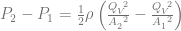
and then

$\Delta P = \frac{1}{2}\rho Q_v^{\ 2}\left(\frac{1}{A_2^{\ 2}} - \frac{1}{A_1^{\ 2}}\right)$

giving

$\Delta P = \frac{1}{2}\rho Q_v^{\ 2}\frac{1}{A_2^{\ 2}}\left(1 - \frac{A_2^{\ 2}}{A_1^{\ 2}}\right)$ .

This is readily solved for $Q_V$

$Q_V = \sqrt{\frac{2\Delta P}{\rho}}\times\left(\frac{A_2}{\sqrt{1-\left(\frac{A_2}{A_1}\right)^2}}\right)$ .

Going through this hoopla teaches us a couple things. One important thing is that the volumetric flow rate—the quantity we need to increase—depends on the pressure difference between the tube and the orifice in a nonlinear fashion. It also tells us that the only way to increase the flow rate is to either increase the pressure differential or, make $A_1 = A_2$ . Making the cross-sectional areas the same is impossible due to our valve constraints however, we can make them as close as possible. Danielle, can you do some calculations on comparing the difference between varying the pressure differential the areas and see which coefficient gives us the greatest boost in volumetric flow?

Inspecting the above equation also taught me an analog to vacuum and current. If I have a wire and I put current through it, the electrons will happily move along the wire with no problem. But, if I add a resistor to the wire, the rate at which the electrons move down the wire is changed. The same thing happens in our vacuum tube when air flow meets a change in diameter. The fluid flow hits a resistance and thus slows the bulk fluid motion down if the diameter is decreased.

This is good. And yes, you were right Damian. This of course means that you (Damian) are going to need to figure out a way to pull a better vacuum on the tube.

12 Comments

ALP Friday 2012-11-2

Posted by () in Open Notebook Science on November 4, 2012

On Friday Danielle and I worked on the vacuum tube a bit. We replaced the regulator for a ball valve and noticed that the flow through the Aerolizer increased from the previously stated 45L/min to about 75L/min. While this is an improvement, we need to get it up to 90L/min.

Once we can get it to 90L/min, we will need to ensure that it maintains that level of airflow for at least 4 seconds. That may require us to add length to the tube which should be fine.

Finally, we need to get some more fittings for the tube. I’ll attempt to go to the hardware store to find some.

Leave a comment

ALP testing vacuum

Posted by () in Open Notebook Science on October 28, 2012

On Friday 2012-10-27 I was able to play around with the vacuum tube. Gio and I set it up to pull a vacuum and were able to get it to work just fine. Below is a video of it working. If the video is not available, it is because Google has for some reason decided that I have to have a Google+ account in order to upload new content to YouTube. Since I have no need for a Google+ account, I deleted it which, may cause the below video to not work since Google want me to have a Google+ account in order to make videos I post publicly available. If it doesn’t work, please let me know in the comments.

I did notice that there is a leak in the port that connects to the vacuum. I believe that this can be fixed with more of the white goop. I also put some vacuum grease by our workstation if someone wanted to try it out.

The next step is to connect one of the regulators to the other side of the tube to see if it will effectively draw in air into the tube when opened. The next step is to hook up the stepper motor to the regulator to see if we can control the vacuum through an Arduino script.

Danielle and Damian, if you guys could hook up the regulator and fix the leak this week, that would be great!

2 Comments

Andy Maloney

sizing lactose 02

sizing lactose 01

Particle sizing

sieving analysis

sieving lactose 03

SuperTab 30GR

Pharmatose 150M

SuperTab 11SD

sieving lactose 02

SuperTab 11SD

Pharmatose 150M

sieving lactose

Introduction

Sieving

SuperTab 30GR

SuperTab 11SD

ALP new vacuum pump

Vacuum pump

Motor control

ALP vacuum notes

ALP Friday 2012-11-2

ALP testing vacuum

Recent Posts

Archives

Categories

Meta