sizing lactose 02

I went ahead and developed my own script to look at the 10th, 50th, and 90th percentiles for the particle sizing done on the SympaTEC HELOS laser diffractor device. As I suspected, the machine does in fact plot the cumulative distribution of particles and fits the data to a Sigmoid. It then calculates the 10th, 50th, and 90th percentiles and reports those values back to a txt file. The script is below the summary table. I will note that I got a NAN for one of the calculated measurements which, caused me to toss out that data point for my calculations. For completeness, I also removed it from the reported values.

Forgive the markdown table below, wordpress doesn’t recognize how to deal with markdown for some reason. It also doesn’t understand what WHITESPACE is supposed to mean. Nonetheless, it is clear that the machine is doing what one would expect as my calculated values are within error of the values reported. This is good as it is no longer a blackbox to me and I will report the values that it gives.

Pharmatose 150M
| Percentile | Reported Average | Reported STD | Calculated Ave | Calculated STD |
|:----------:|:----------------:|:------------:|:--------------:|:--------------:|
| 10th       | 121.9 µm         |  6.6 µm      | 117.1 µm       |  6.5 µm        |
| 50th       | 190.7 µm         | 11.4 µm      | 191.9 µm       | 11.8 µm        |
| 90th       | 268.2 µm         | 22.6 µm      | 260.0 µm       | 20.8 µm        |

SuperTab 11SD
| Percentile | Reported Average | Reported STD | Calculated Ave | Calculated STD |
|:----------:|:----------------:|:------------:|:--------------:|:--------------:|
| 10th       | 119.7 µm         |  7.9 µm      | 116.3 µm       |  6.1 µm        |
| 50th       | 187.9 µm         | 15.1 µm      | 189.1 µm       | 16.6 µm        |
| 90th       | 271.4 µm         | 39.9 µm      | 262.4 µm       | 32.9 µm        |

SuperTab 30GR
| Percentile | Reported Average | Reported STD | Calculated Ave | Calculated STD |
|:----------:|:----------------:|:------------:|:--------------:|:--------------:|
| 10th       | 117.9 µm         | 26.5 µm      | 117.9 µm       | 18.1 µm        |
| 50th       | 183.5 µm         | 21.0 µm      | 189.9 µm       | 13.4 µm        |
| 90th       | 257.4 µm         | 28.3 µm      | 256.4 µm       | 19.2 µm        |

# Import statements.
import numpy as np
from scipy.optimize import curve_fit

# Input data.
size = [ 4.50, 5.50, 6.50, 7.50, 9.00, 11.00, 13.00,
 15.50, 18.50, 21.50, 25.00, 30.00, 37.50, 45.00,
 52.50, 62.50, 75.00, 90.00, 105.00, 125.00, 150.00,
 180.00, 215.00, 255.00, 305.00, 365.00, 435.00, 515.00,
 615.00, 735.00, 875.00 ]

# Pharmatose 150M
pharmatose_150M_od43_63 = [
 2.16, 2.38, 2.54, 2.67, 2.82, 2.96, 3.07,
 3.17, 3.28, 3.37, 3.46, 3.59, 3.77, 3.94,
 4.10, 4.31, 4.67, 5.43, 6.96, 11.20, 21.73,
 41.64, 67.86, 89.30, 100.00, 100.00, 100.00, 100.00,
 100.00, 100.00, 100.00 ]
pharmatose_150M_od08_90 = [
 1.62, 1.87, 2.08, 2.26, 2.49, 2.73, 2.91,
 3.08, 3.20, 3.27, 3.27, 3.27, 3.27, 3.27,
 3.35, 3.52, 3.80, 4.40, 5.81, 10.75, 25.32,
 51.46, 81.69, 97.52, 100.00, 100.00, 100.00, 100.00,
 100.00, 100.00, 100.00 ]
pharmatose_150M_od15_83 = [
 2.27, 2.49, 2.63, 2.74, 2.84, 2.93, 2.93,
 2.93, 2.93, 2.93, 2.93, 2.93, 2.93, 2.93,
 3.01, 3.13, 3.36, 3.92, 5.31, 9.84, 21.84,
 42.60, 67.85, 88.46, 99.02, 100.00, 100.00, 100.00,
 100.00, 100.00, 100.00 ]
pharmatose_150M_od15_52 = [
 1.69, 1.90, 2.06, 2.18, 2.33, 2.47, 2.57,
 2.57, 2.57, 2.57, 2.57, 2.57, 2.57, 2.57,
 2.68, 2.81, 2.98, 3.38, 4.42, 8.12, 18.74,
 38.48, 63.38, 84.92, 94.39, 96.65, 100.00, 100.00,
 100.00, 100.00, 100.00 ]
pharmatose_150M_od09_31 = [
 2.25, 2.54, 2.77, 2.96, 3.17, 3.38, 3.53,
 3.66, 3.77, 3.84, 3.84, 3.84, 3.84, 3.92,
 4.05, 4.25, 4.55, 5.26, 7.09, 13.46, 29.42,
 53.34, 79.60, 94.53, 100.00, 100.00, 100.00, 100.00,
 100.00, 100.00, 100.00 ]
pharmatose_150M_od21_24 = [
 2.29, 2.53, 2.70, 2.82, 2.94, 3.03, 3.03,
 3.03, 3.03, 3.03, 3.03, 3.09, 3.23, 3.38,
 3.53, 3.73, 4.07, 4.78, 6.38, 11.15, 22.47,
 40.47, 61.63, 80.36, 94.20, 100.00, 100.00, 100.00,
 100.00, 100.00, 100.00 ]
pharmatose_150M_od13_58 = [
 2.42, 2.66, 2.82, 2.93, 3.05, 3.14, 3.14,
 3.14, 3.14, 3.14, 3.14, 3.14, 3.14, 3.14,
 3.22, 3.36, 3.60, 4.11, 5.23, 8.67, 18.17,
 36.99, 62.47, 83.56, 94.95, 100.00, 100.00, 100.00,
 100.00, 100.00, 100.00 ]
pharmatose_150M_od07_26 = [
 3.11, 3.51, 3.81, 4.03, 4.27, 4.48, 4.60,
 4.70, 4.70, 4.70, 4.70, 4.76, 4.87, 5.04,
 5.25, 5.57, 6.03, 6.97, 9.19, 16.09, 32.51,
 57.07, 81.43, 94.38, 100.00, 100.00, 100.00, 100.00,
 100.00, 100.00, 100.00 ]
pharmatose_150M_od15_40 = [
 2.57, 2.90, 3.15, 3.33, 3.51, 3.66, 3.75,
 3.75, 3.75, 3.75, 3.75, 3.80, 3.92, 4.06,
 4.19, 4.36, 4.59, 5.09, 6.23, 9.78, 19.14,
 36.31, 58.95, 82.39, 98.64, 100.00, 100.00, 100.00,
 100.00, 100.00, 100.00 ]
pharmatose_150M_od16_94 = [
 2.60, 2.89, 3.09, 3.22, 3.35, 3.44, 3.44,
 3.44, 3.44, 3.44, 3.44, 3.53, 3.66, 3.77,
 3.87, 4.02, 4.26, 4.73, 5.79, 9.07, 17.62,
 33.27, 53.49, 73.69, 89.55, 97.91, 100.00, 100.00,
 100.00, 100.00, 100.00 ]

pharmatose_150M_ave = [np.average(item) for item in
 zip(pharmatose_150M_od43_63, pharmatose_150M_od08_90,
 pharmatose_150M_od15_83, pharmatose_150M_od15_52,
 pharmatose_150M_od09_31, pharmatose_150M_od21_24,
 pharmatose_150M_od13_58, pharmatose_150M_od07_26,
 pharmatose_150M_od15_40, pharmatose_150M_od16_94)]
pharmatose_150M_std = [np.std(item) for item in
 zip(pharmatose_150M_od43_63, pharmatose_150M_od08_90,
 pharmatose_150M_od15_83, pharmatose_150M_od15_52,
 pharmatose_150M_od09_31, pharmatose_150M_od21_24,
 pharmatose_150M_od13_58, pharmatose_150M_od07_26,
 pharmatose_150M_od15_40, pharmatose_150M_od16_94)]

pharmatose_150M = [ pharmatose_150M_od43_63, pharmatose_150M_od08_90,
 pharmatose_150M_od15_83, pharmatose_150M_od15_52,
 pharmatose_150M_od09_31, pharmatose_150M_od21_24,
 pharmatose_150M_od13_58, pharmatose_150M_od07_26,
 pharmatose_150M_od15_40, pharmatose_150M_od16_94 ]

# SuperTab 11SD
supertab_11SD_od20_93 = [
 0.43, 0.50, 0.57, 0.63, 0.71, 0.81, 0.90,
 0.99, 1.10, 1.19, 1.29, 1.43, 1.65, 1.88,
 2.13, 2.49, 3.07, 4.27, 6.70, 13.32, 29.17,
 56.35, 84.37, 100.00, 100.00, 100.00, 100.00, 100.00,
 100.00, 100.00, 100.00 ]
supertab_11SD_od12_18 = [
 0.55, 0.61, 0.61, 0.61, 0.61, 0.61, 0.61,
 0.61, 0.61, 0.61, 0.68, 0.80, 0.99, 1.21,
 1.45, 1.81, 2.36, 3.43, 5.67, 12.27, 28.07,
 53.28, 81.44, 100.00, 100.00, 100.00, 100.00, 100.00,
 100.00, 100.00, 100.00 ]
supertab_11SD_od08_01 = [
 0.00, 0.07, 0.07, 0.07, 0.07, 0.07, 0.07,
 0.07, 0.07, 0.07, 0.16, 0.30, 0.54, 0.83,
 1.15, 1.63, 2.41, 3.92, 6.94, 15.44, 33.55,
 58.19, 83.75, 97.68, 100.00, 100.00, 100.00, 100.00,
 100.00, 100.00, 100.00 ]
supertab_11SD_od06_29 = [
 0.00, 0.06, 0.06, 0.06, 0.06, 0.06, 0.06,
 0.06, 0.06, 0.06, 0.15, 0.31, 0.56, 0.83,
 1.12, 1.53, 2.09, 2.92, 4.35, 8.68, 20.48,
 40.37, 63.77, 85.46, 99.23, 100.00, 100.00, 100.00,
 100.00, 100.00, 100.00 ]
supertab_11SD_od15_59 = [
 0.00, 0.06, 0.06, 0.06, 0.06, 0.06, 0.06,
 0.06, 0.06, 0.06, 0.16, 0.32, 0.59, 0.88,
 1.18, 1.59, 2.17, 3.14, 4.93, 9.76, 21.00,
 38.97, 60.11, 79.39, 94.27, 100.00, 100.00, 100.00,
 100.00, 100.00, 100.00 ]
supertab_11SD_od10_27 = [
 0.00, 0.06, 0.06, 0.06, 0.06, 0.06, 0.06,
 0.06, 0.06, 0.06, 0.14, 0.27, 0.49, 0.74,
 0.98, 1.29, 1.69, 2.39, 3.84, 8.10, 18.11,
 34.17, 53.57, 71.78, 85.51, 94.19, 100.00, 100.00,
 100.00, 100.00, 100.00 ]
supertab_11SD_od09_51 = [
 0.61, 0.76, 0.90, 1.04, 1.24, 1.51, 1.75,
 2.03, 2.32, 2.57, 2.85, 3.25, 3.86, 4.46,
 4.99, 5.60, 6.31, 7.52, 10.15, 17.87, 34.59,
 58.89, 83.86, 100.00, 100.00, 100.00, 100.00, 100.00,
 100.00, 100.00, 100.00 ]
supertab_11SD_od07_94 = [
 0.52, 0.60, 0.60, 0.60, 0.60, 0.60, 0.60,
 0.70, 0.81, 0.92, 1.04, 1.21, 1.50, 1.81,
 2.14, 2.61, 3.26, 4.33, 6.32, 11.81, 24.04,
 42.31, 63.21, 81.04, 92.89, 100.00, 100.00, 100.00,
 100.00, 100.00, 100.00 ]
supertab_11SD_od08_40 = [
 0.51, 0.59, 0.59, 0.59, 0.59, 0.59, 0.59,
 0.59, 0.59, 0.69, 0.82, 1.01, 1.32, 1.63,
 1.93, 2.31, 2.80, 3.64, 5.22, 9.51, 19.31,
 34.87, 53.46, 71.73, 86.80, 96.02, 100.00, 100.00,
 100.00, 100.00, 100.00 ]

supertab_11SD_ave = [np.average(item) for item in
 zip(supertab_11SD_od20_93, supertab_11SD_od12_18,
 supertab_11SD_od08_01, supertab_11SD_od06_29,
 supertab_11SD_od15_59, supertab_11SD_od10_27,
 supertab_11SD_od09_51, supertab_11SD_od07_94,
 supertab_11SD_od08_40) ]
supertab_11sd_std = [np.std(item) for item in
 zip(supertab_11SD_od20_93, supertab_11SD_od12_18,
 supertab_11SD_od08_01, supertab_11SD_od06_29,
 supertab_11SD_od15_59, supertab_11SD_od10_27,
 supertab_11SD_od09_51, supertab_11SD_od07_94,
 supertab_11SD_od08_40)]

supertab_11SD = [ supertab_11SD_od20_93, supertab_11SD_od12_18,
 supertab_11SD_od08_01, supertab_11SD_od06_29,
 supertab_11SD_od15_59, supertab_11SD_od10_27,
 supertab_11SD_od09_51, supertab_11SD_od07_94,
 supertab_11SD_od08_40 ]

# SuperTab 30GR
supertab_30GR_od05_40 = [
 0.89, 0.96, 0.96, 0.96, 0.96, 0.96, 0.96,
 0.96, 0.96, 0.96, 0.96, 0.96, 1.03, 1.14,
 1.26, 1.43, 1.63, 1.90, 2.53, 4.99, 13.15,
 30.51, 55.09, 80.77, 98.84, 100.00, 100.00, 100.00,
 100.00, 100.00, 100.00 ]
supertab_30GR_od14_59 = [
 0.82, 0.91, 0.91, 0.91, 0.91, 0.91, 0.91,
 0.91, 0.91, 0.91, 0.99, 1.11, 1.29, 1.47,
 1.64, 1.88, 2.23, 2.82, 3.96, 7.42, 17.30,
 37.26, 64.08, 86.29, 97.81, 100.00, 100.00, 100.00,
 100.00, 100.00, 100.00 ]
supertab_30GR_od14_16 = [
 0.81, 0.90, 0.90, 0.90, 0.90, 0.90, 0.90,
 0.90, 0.90, 0.90, 0.97, 1.07, 1.23, 1.40,
 1.57, 1.83, 2.19, 2.83, 4.08, 8.10, 19.27,
 38.78, 62.03, 80.56, 93.90, 100.00, 100.00, 100.00,
 100.00, 100.00, 100.00 ]
supertab_30GR_od12_68 = [
 1.11, 1.23, 1.32, 1.32, 1.32, 1.32, 1.32,
 1.32, 1.32, 1.32, 1.41, 1.55, 1.76, 2.01,
 2.29, 2.71, 3.30, 4.15, 5.64, 10.08, 22.32,
 43.58, 68.81, 86.73, 96.04, 99.37, 100.00, 100.00,
 100.00, 100.00, 100.00 ]
supertab_30GR_od19_84 = [
 1.08, 1.19, 1.28, 1.28, 1.28, 1.28, 1.28,
 1.28, 1.28, 1.28, 1.37, 1.50, 1.70, 1.91,
 2.14, 2.45, 2.89, 3.59, 4.96, 9.26, 21.13,
 42.65, 69.46, 90.32, 100.00, 100.00, 100.00, 100.00,
 100.00, 100.00, 100.00 ]
supertab_30GR_od16_64 = [
 1.34, 1.48, 1.59, 1.68, 1.78, 1.88, 1.97,
 1.97, 1.97, 2.06, 2.16, 2.30, 2.52, 2.75,
 2.98, 3.30, 3.73, 4.44, 5.85, 10.46, 23.76,
 47.74, 76.14, 92.11, 97.37, 100.00, 100.00, 100.00,
 100.00, 100.00, 100.00 ]
supertab_30GR_od07_38 = [
 8.09, 9.59, 10.86, 11.92, 13.20, 14.50, 15.46,
 6.35, 17.12, 17.71, 18.27, 18.98, 20.05, 21.20,
 2.48, 24.29, 26.55, 29.80, 34.86, 45.30, 62.11,
 80.83, 93.74, 100.00, 100.00, 100.00, 100.00, 100.00,
 100.00, 100.00, 100.00 ]
supertab_30GR_od22_13 = [
 1.32, 1.48, 1.60, 1.70, 1.82, 1.93, 2.02,
 2.12, 2.12, 2.21, 2.32, 2.46, 2.68, 2.90,
 3.14, 3.47, 3.93, 4.70, 6.09, 10.07, 20.37,
 38.47, 60.39, 79.95, 92.87, 98.84, 100.00, 100.00,
 100.00, 100.00, 100.00 ]
supertab_30GR_od14_21 = [
 1.99, 2.23, 2.41, 2.56, 2.74, 2.92, 3.06,
 3.20, 3.34, 3.46, 3.59, 3.78, 4.06, 4.36,
 4.65, 5.03, 5.49, 6.19, 7.54, 11.87, 24.41,
 48.74, 80.55, 98.71, 100.00, 100.00, 100.00, 100.00,
 100.00, 100.00, 100.00 ]
supertab_30GR_od09_15 = [
 3.94, 4.61, 5.17, 5.65, 6.22, 6.80, 7.23,
 7.62, 7.97, 8.25, 8.53, 8.89, 9.44, 10.01,
 10.60, 11.41, 12.38, 13.78, 16.37, 23.89, 41.22,
 66.35, 88.63, 98.00, 100.00, 100.00, 100.00, 100.00,
 100.00, 100.00, 100.00 ]

supertab_30GR_ave = [np.average(item) for item in
 zip(supertab_30GR_od05_40, supertab_30GR_od14_59,
 supertab_30GR_od14_16, supertab_30GR_od12_68,
 supertab_30GR_od19_84, supertab_30GR_od16_64,
 supertab_30GR_od07_38, supertab_30GR_od22_13,
 supertab_30GR_od14_21, supertab_30GR_od09_15) ]
supertab_30GR_std = [np.std(item) for item in
 zip(supertab_30GR_od05_40, supertab_30GR_od14_59,
 supertab_30GR_od14_16, supertab_30GR_od12_68,
 supertab_30GR_od19_84, supertab_30GR_od16_64,
 supertab_30GR_od07_38, supertab_30GR_od22_13,
 supertab_30GR_od14_21, supertab_30GR_od09_15) ]

supertab_30GR = [ supertab_30GR_od05_40, supertab_30GR_od14_59,
 supertab_30GR_od14_16, supertab_30GR_od12_68,
 supertab_30GR_od19_84, supertab_30GR_od16_64,
 supertab_30GR_od22_13,
 supertab_30GR_od14_21, supertab_30GR_od09_15 ]

# Define the Sigmoidal function.
def sigmoid(x, a, b, k, t):
 """ Sigmoidal function.
 x = Input data.
 a = Minimum value of input data.
 b = Maximum value of input data.
 k = Midpoint of the Sigmoid.
 t = Rate of increase.
 """
 y = a + (b/(1 + np.exp((k - x)/t)))
 return y

# Get the 10, 50, and 90th percentiles.
pharmatose_150M_percentiles = []
for item in pharmatose_150M:
 popt, pcov = curve_fit(sigmoid, size, item)
 _10 = popt[2] - popt[3]*np.log(popt[1]/(10 - popt[0]) - 1)
 _50 = popt[2] - popt[3]*np.log(popt[1]/(50 - popt[0]) - 1)
 _90 = popt[2] - popt[3]*np.log(popt[1]/(90 - popt[0]) - 1)
 temp = _10, _50, _90
 pharmatose_150M_percentiles.append(temp)
supertab_11SD_percentiles = []
for item in supertab_11SD:
 popt, pcov = curve_fit(sigmoid, size, item)
 _10 = popt[2] - popt[3]*np.log(popt[1]/(10 - popt[0]) - 1)
 _50 = popt[2] - popt[3]*np.log(popt[1]/(50 - popt[0]) - 1)
 _90 = popt[2] - popt[3]*np.log(popt[1]/(90 - popt[0]) - 1)
 temp = _10, _50, _90
 supertab_11SD_percentiles.append(temp)
supertab_30GR_percentiles = []
for item in supertab_30GR:
 popt, pcov = curve_fit(sigmoid, size, item)
 _10 = popt[2] - popt[3]*np.log(popt[1]/(10 - popt[0]) - 1)
 _50 = popt[2] - popt[3]*np.log(popt[1]/(50 - popt[0]) - 1)
 _90 = popt[2] - popt[3]*np.log(popt[1]/(90 - popt[0]) - 1)
 temp = _10, _50, _90
 supertab_30GR_percentiles.append(temp)

# Create a list of the generated percentile values.
pharmatose_150M_10 = [ 119.34, 121.96, 125.33, 129.43, 114.13, 120.18, 128.50,
 107.36, 125.58, 127.73 ]
pharmatose_150M_50 = [ 191.16, 178.32, 190.26, 196.19, 175.81, 195.76, 197.87,
 171.37, 201.16, 208.96 ]
pharmatose_150M_90 = [ 258.28, 236.00, 262.29, 281.83, 242.86, 289.82, 283.27,
 241.46, 278.42, 308.22 ]
pharmatose_150M_reported = [ pharmatose_150M_10, pharmatose_150M_50,
 pharmatose_150M_90 ]

supertab_11SD_10 = [ 114.96, 118.13, 112.20, 127.81, 125.54, 129.74, 104.16, 118.42, 126.26 ]
supertab_11SD_50 = [ 172.99, 176.09, 170.03, 194.41, 198.26, 208.57, 169.02, 192.88, 208.49 ]
supertab_11SD_90 = [ 229.41, 233.45, 232.95, 271.49, 290.66, 336.04, 230.22, 292.81, 325.82 ]
supertab_11SD_reported = [ supertab_11SD_10, supertab_11SD_50,
 supertab_11SD_90 ]

supertab_30GR_10 = [ 140.35, 131.52, 129.25, 124.65, 126.56, 123.02,
 124.67, 116.38, 44.88 ] # 5.82
supertab_30GR_50 = [ 207.76, 196.63, 196.89, 188.90, 189.60, 182.79, 131.99, 198.41, 181.39, 160.48 ]
supertab_30GR_90 = [ 280.54, 271.11, 290.39, 272.56, 254.39, 249.72, 204.86, 293.91, 235.82, 220.86 ]
supertab_30GR_reported = [ supertab_30GR_10, supertab_30GR_50,
 supertab_30GR_90 ]

for i in range(0, 3):
 rept_ave = np.average(pharmatose_150M_reported[i])
 calc_ave = np.average([item[i] for item in pharmatose_150M_percentiles])
 rept_std = np.std(pharmatose_150M_reported[i])
 calc_std = np.std([item[i] for item in pharmatose_150M_percentiles])
 print 'Calculated average for Pharmatose 150M = %f' % calc_ave
 print 'Reported average for Pharmatose 150M = %f' % rept_ave
 print 'Calculated STD for Pharmatose 150M = %f' % calc_std
 print 'Reported STD for Pharmatose 150M = %f' % rept_std

for i in range(0, 3):
 rept_ave = np.average(supertab_11SD_reported[i])
 calc_ave = np.average([item[i] for item in supertab_11SD_percentiles])
 rept_std = np.std(supertab_11SD_reported[i])
 calc_std = np.std([item[i] for item in supertab_11SD_percentiles])
 print 'Calculated average for SuperTab 11SD = %f' % calc_ave
 print 'Reported average for SuperTab 11SD = %f' % rept_ave
 print 'Calculated STD for SuperTab 11SD = %f' % calc_std
 print 'Reported STD for SuperTab 11SD = %f' % rept_std

for i in range(0, 3):
 rept_ave = np.average(supertab_30GR_reported[i])
 calc_ave = np.average([item[i] for item in supertab_30GR_percentiles])
 rept_std = np.std(supertab_30GR_reported[i])
 calc_std = np.std([item[i] for item in supertab_30GR_percentiles])
 print 'Calculated average for SuperTab 30GR = %f' % calc_ave
 print 'Reported average for SuperTab 30GR = %f' % rept_ave
 print 'Calculated STD for SuperTab 30GR = %f' % calc_std
 print 'Reported STD for SuperTab 30GR = %f' % rept_std

sizing lactose 01

Particle sizing

I was able to size the lactose particles after sieving using the SympaTEC HELOS laser diffractor in the lab. I unfortunately had to do this step multiple times as I was having some difficulty interpreting the results. Nonetheless, I believe I understand how the device works now.

The sizer uses a laser to illuminate particles that are suspended in mineral oil that has 1% Span-85 in it. The laser is collimated and has a beam width of about 2 cm. A lens is then used to focus the light from the sample onto a detector. The detector is placed in the Fourier plane of the lens in order to detect diffraction patterns from the particles. Using Fraunhofer diffraction theory, a particle size is estimated from its diffraction pattern.

What caused my initial hesitation about the results was that I was told to not put a lot of particles in the cuvette—so I didn’t. However, I was told to add more particles to the cuvette and take successive measurements. I found documentation on the computer that states one should shoot for a 10–15% optical density which, at the time of my first run with the machine, I had no clue as to what that meant. My main cause of confusion and why I redid the sizing was when I added particles to the cuvette, it caused the sizing results to shift slightly.

My second go with the machine allowed for more clarity. I understand the caution for not putting a ton of particles in the cuvette since you don’t want to saturate the detector. If there are too many particles, than the detector (which I’m assuming is nothing more than a camera with multiple arrays) is unable to detect individual diffraction patterns through the software. I did oversaturate the detector once but, I just waited a couple of minutes till the particles settled in the cuvette. I then retook the measurement and sure enough, the detector wasn’t saturated. Of course doing this skews the particle size results as the detector is detecting particles small enough that stayed in solution. The sizer indicates the “optical density” of a measurement and I believe this is a measure of the turbidity of the solution in the cuvette. I was able to get it as high as 44% optical density without the software complaining.

The data I obtained shifted dependent upon the time in which particles were allowed to be in the cuvette—i.e. larger ones sank. So, I made sure to load the cuvette with tons of particles, wait till it was able to detect them, and then took measurements as particles sunk. I also added particles to the cuvette over time adding small amounts as was instructed for me to do. Doing this gave a spread in sizing that I’m assuming comes from a spread in particles after sieving.

The SympaTEC software gives a plot of sizing data and shows the 10th, 50th, and 90th percentile of the sizes. I believe it is doing this by fitting a Sigmoid to the size data and finding on the curve the corresponding percentiles. This data is of course plotted in a proprietary .bmp format that is completely useless. So, I’m working on a script to plot the data which, thankfully was output in a txt file. For all intents and purposes I believe using the data that was output by the device is sufficient for sizing purposes. I’m just wanting to have a little fun with the data it gave me.

sieving analysis

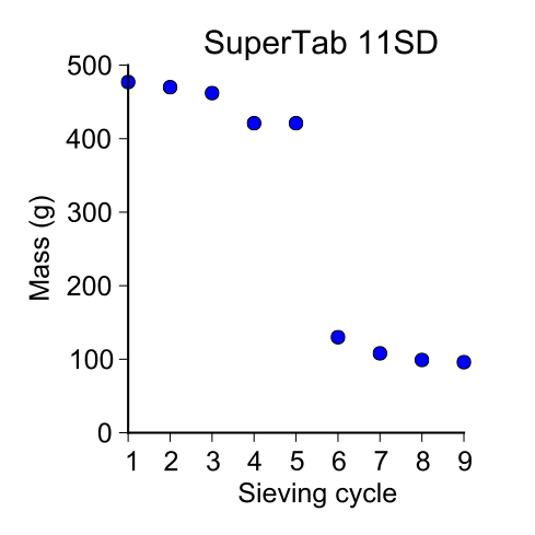
I finished my sieving analysis and writeup for it. Below is the python script that I used to plot the data shown in the graphs below. I don’t know why but wordpress is removing my white space formatting.

# Import statements.
 import matplotlib.pyplot as plt
 from matplotlib import rcParams

# Change the figure size and font used.
 rcParams['font.sans-serif'] = 'Arial'
 rcParams['figure.figsize'] = [3.27, 3.27]
 rcParams['xtick.direction'] = 'out'
 rcParams['ytick.direction'] = 'out'

# Input data. Values are in grams.
 pharmatose150M = [ 205, 165, 103, 90, 85, 81, 81, 78, 75 ]
 supertab11SD = [ 477, 470, 462, 421, 421, 130, 108, 99, 96 ]
 supertab30GR = [ 246, 239, 236, 234, 218, 209, 202, 200 ]

# Generate the x-axis.
 sieve_cycle = [ 1, 2, 3, 4, 5, 6, 7, 8, 9 ]

# Plot the data.
 def plot_data(x, y, marker_type, marker_size, x_label, y_label, title):
 """ Plots the input data.
 x = x-data
 y = y-data
 marker_type = Marker type of the plot.
 marker_size = Marker size of the plot.
 x_label = x-axis label.
 y_label = y-axis label.
 title = Title of the plot.
 """
 # Initialize a figure.
 fig = plt.figure()
 ax = fig.add_subplot(1, 1, 1)
 # Add labels.
 ax.set_xlabel(x_label)
 ax.set_ylabel(y_label)
 ax.set_title(title)
 # Fix the x-axis limit.
 ax.set_xlim([1, 10])
 # Modify the spines so that the top and right spines are not visible.
 ax.xaxis.set_ticks_position('bottom')
 ax.yaxis.set_ticks_position('left')
 ax.spines['right'].set_visible(False)
 ax.spines['top'].set_visible(False)
 ax.spines['left'].set_smart_bounds(True)
 ax.spines['bottom'].set_smart_bounds(True)
 #ax.spines['left'].set_position(('axes', -0.01))
 # Plot the data.
 data = ax.plot(x, y, marker_type, marker_size)
 for artist in data:
 artist.set_clip_on(False)
 fig.tight_layout()
 fig.savefig(title.lower().replace(' ', '') + '.pdf')

plot_data(sieve_cycle, pharmatose150M, 'o', 3, 'Sieve cycle', 'Mass (g)',
 'Pharmatose 150M')
 plot_data(sieve_cycle, supertab11SD, 'o', 3, 'Sieve cycle', 'Mass (g)',
 'SuperTab 11SD')
 plot_data(sieve_cycle[:-1], supertab30GR, 'o', 3, 'Sieve cycle', 'Mass (g)',
 'SuperTab 30GR')

sieving lactose 03

Last time I did a bulk sieving of the powders in order to fractionate them into different distributions of grain sizes. From this initial sieving, I saw that the largest amount of powder in each of the sieved sizes was the 125–150 µm range. If the Pharmatose 150M lactose took approximately the same number of sieving cycles as the SuperTabs than I wouldn’t be doing this extra sieving step, however, because it took 8 cycles I am not convinced that the sieving is complete enough to give large cutoffs for the 125–150 µm size range. This is why I have decided to sieve each of the 125–150 µm sizes again to ensure that sieving is producing a strong cutoff between sizes. Like before, I’ve set up the following sieves:

• Lid
• 250 µm
• 125 µm
• 75 µm
• Bucket

this time ignoring the 45 µm sieve since it has a hole in it. I put the 125–150 µm size range in the top sieve and let it shake for 30 minutes. I’m only interested in the 125–250 µm range so this is the only one that I will be measuring.

SuperTab 30GR

Initial conditions:

• 2014-05-04
• Temperature = 22.9˚C
• Relative humidity = 22%

My first sieving for the second sieve cycle was:

• 125–250 µm = 218 g

I’ll note that the powder seemed to be have somewhat of a charge to it and as such, seemed to cling to the sieve. As seen in a previous post, this weight is significantly different than the one I ended with so, time for another sieve cycle.

My second sieving for the second sieve cycle was:

• 125–250 µm = 209 g

My third sieving for the second sieve cycle was:

• 125–250 µm = 202 g

My fourth sieving for the second sieve cycle was:

• 125–250 µm =  200 g

Pharmatose 150M

My first sieving for the second sieve cycle was:

• 125–250 µm = 75 g

Since the last sieving of the Pharmatose 150M was at 78 g, this change is within the 1–5% weight change and thus I will not be sieving it more.

SuperTab 11SD

I separated the SuperTab 125–250 µm fraction because it was quite large. So I started off with about 150 g of it in the sievers.

My first sieving for the second sieve cycle was:

• 125–250 µm = 130 g

My second sieving for the second sieve cycle was:

• 125–250 µm = 108 g

My third sieving for the second sieve cycle was:

• 125–250 µm = 99 g

My fourth sieving for the second sieve cycle was:

• 125–250 µm = 96 g

The powders are now within the arbitrarily decided 1–5% change of weight between sieving cycles. The next step is to size the particles to see if they actually are within these ranges.