Measuring tap densities

We have devised an apparatus that allows visualization of powder compactions for individual taps. The device has been in a state of constant flux as we try to iron out the bugs in the system and I will update my notebook with a description of the build soon. Up till now, most of our time has been building the device and making sure it works properly. Recently we were able to get data and both Damian and I have been working on building a script that programmatically calculates the distance powder compacts with each tap. While Damian and I are working on the same thing, his approach is very different and I must admit, I’m intrigued by his logic. Hopefully our scripts will output the same thing because if they don’t, we will have to debug things.

Below is a script that I have written in Octave. It should function fine in MatLab as well.

% Generate a list containing the names of the files to be analyzed.
fileDirectory = 'PATH/TO/DIRECTORY/';
filePattern = fullfile(fileDirectory, '*.png');
dataFiles = dir(filePattern);
baseFileName = {dataFiles.name}';
fullFileName = strcat(fileDirectory, '/', baseFileName);

plotDirectory = 'PATH/TO/PUT/PLOTS';
pixels = 56;
cutoffValue = 14000;
lactose = 'pharmatose125M';
sizeRange = '--63-150um';
trial = '--trial01';

saveName = strcat(lactose, sizeRange, trial);
plotTitle = saveName;

% Open the image file and obtain the roi.
for j = 1:numel(fullFileName)
 x = [ 0:1:250 ];
 image = imread(sprintf('%s', fullFileName{j}));
 roi = image(130:255, 225:475);
 [ m n ] = size(roi);
 for i = 1:n
 pixelSum(i) = sum(roi(:,i));
 endfor
 cutoff = [ x; pixelSum ]';
 ind = find(cutoff(:,2) >= cutoffValue);
 tap(j) = ind(1)*(1.27/pixels);
 tapY(j) = cutoff(ind(1), 2);
 X = x*(1.27/pixels);
 figure(j);
 subplot(2,1,1);
 imshow(image);
 subplot(2,1,2);
 hold on;
 plot(X, pixelSum, 'LineWidth', 1.2, 'b');
 plot(tap(j), tapY(j), 'ks', 'markersize', 10)
 xlabel('Distance (cm)');
 ylabel('Intensity (arb. units)');
 axis([0, 6, 8000, 26000])
 title(strcat(plotTitle, sprintf('--%04d.png', j)));
 legend('Pixel intensity values.', 'Point where the end of the shadow is defined.');
 set (gca, "xminortick", "on", "yminortick", "off")
 print(strcat(plotDirectory, strcat(saveName, sprintf('--%04d.png', j))))
 hold off;
 delete(j);
endfor

figure();
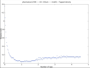
plot(X(1:201), tap, 'b.');
title(strcat(lactose, '--', sizeRange, '--', trial, '--Tapped density'));
xlabel('Number of taps')
ylabel('Distance (cm)')

The script will open .png files in the specified directory. The raw data looks like the figure below.

There is a ruler—top vertical bar—that is used to determine pixel sizes in the analysis. The ruler let us know that for (this set of images) 56 pixels equaled 1.27cm. Obviously the image is on its side and gravity is pointing to the left. This statement will become obvious in a later post. Nonetheless, these are what the raw image files look like.

Processing the images entails selecting a region of interest (ROI), summing all the pixel values (column-wise) in the ROI, and selecting the pixel value along the horizontal direction in the raw image where the summed pixel intensity is above some threshold. I have made the script output each plot which, increases the computation cost but I think is essential to ensuring the final output graph is okay or not. The intermediate processed graph looks like the image below.

Where I have ensured that the original image is attached to the pixel intensity graph for clarity. Just for fun, and to see if WordPress would allow me to do it, I have made an animated gif that shows the complete run of taps we performed. In order to visualize it, you need to click on the image and it will run in a new browser window—tested on Chrome.

Ultimately we are interested in compaction versus taps and the above script does give that output. There is still some massaging to be done with the script and the outputs of the graphs. I think I will want to do some analysis in qtiplot as well so the output will need to save the data appropriately. Nonetheless, here is the final graph that I was initially interested in producing.

Thanks again everyone for their help, suggestions, data taking and time working on this.

Tap densities

First, I’d like to thank all the students for transitioning to WordPress. From what I can tell, OpenWetWare is not being developed any more and from my standpoint, should not be used. I will have to figure out a way to move notebook entries written there to WordPress for both me and Sarah.

Tumblr is a great blog type service and there is nothing wrong with it. I just felt that we should all be on the same page when it comes to notebook. Plus, WordPress will email when a notebook entry has been made. This is ideal for me and anyone that is working on multiple projects and wants to stay connected with the people updating things.

Thanks again everyone!